There is a foundation of transcription for human cell types
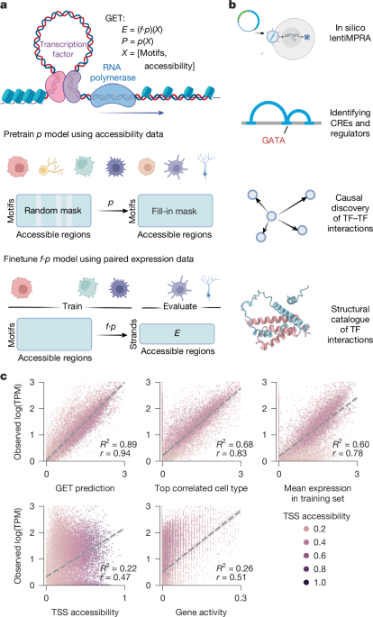
Learning regulatory grammar in the GET architecture using high-dimensional chromatin accessibility data from a variety of human cell types: the lentiMPRA model
The model underwent 800 training epochs, lasting 1 week. This extensive training period was essential for the model to learn the regulatory grammar from chromatin accessibility data across a wide array of human cell types.
There are three parts to theGET architecture, including a regulatory element embedding layer, a regulatory element-wise attention layer, and a linear output layer. GET takes 200 regulatory elements, each with 282 motif binding scores and optionally one accessibility score as an input sample. The input is a matrix of 200. When we choose to not use the quantitative accessibility score, we set the values in the 283-th column to 1.
The K562 lentiMPRA elements were grouped by using the data from histone mark and other data. We selected the elements overlapping with states ‘12 EnhBiv’, ‘6 EnhG’ and ‘7 Enh’ as enhancers, and those overlapping with ‘13 ReprPC’, ‘14 ReprPCWk’ and ‘15 Quies’ as repressive and quiescent regions.
Visualizing the Jacobian of a genome-wide gene-by-motif matrix for cell type c,Vc with application to GATA
The Jacobian matrix (tensor) JX ∈ ({{\mathbb{R}}}^{r\times 2\times r\times m}) of (f) at the point (E, X) evaluates how each output dimension will change when each input dimension changes by a small quantity. The strand and output dimensions are picked based on the given gene.
The feature (motif) importance vector ({{\rm{v}}}_{g}\in {{\mathbb{R}}}^{m}) is obtained by multiplying the gradient element-wise with the original input and summarizing across regions:
where (\odot ) signifies the element-wise or Hadamard product. The matrix is mostly used for feature interaction analysis and we use it with quantitative ATAC signal when using a model. This facilitates study of the relationship between regulators and observed chromatin accessibility.
The cell-type-specific genome-wide gene-by-motif matrix for cell type c, Vc is acquired by concatenating the ({{\rm{v}}}_{g}) across the genome. Different cell types can be applied the same process.
We use the Jacobian of the region to calculate the importance score, as it is less skewed than the input score and makes the Jacobian more comparable across regions. The per-region Jacobian score is normalized by the maximum score per gene to make scores comparable across genes with different expression levels.
In the case of GATA, we can ask which genes will be most affected by this TFF by looking at the largest entries in the motif column. The top 1000 genes were chosen, and we did our enrichment analysis using g:Profiler and g.Scs multiple hypothesis testing correction. We filtered the results using term size (gene number in a term definition) greater than 500 and less than 1,000. Significant terms were retained if the P value was less than 0.05. We further selected TFs in the ‘Hemopoiesis’ term with expression log10(TPM > 1) for visualization against the GATA motif score.
In this analysis, we sought to elucidate the relationships between TFs and expression of their target genes across different cell types. The files were grouped into a single structure, consisting of genes, motifs and cell features. We figured out the mean expression levels of the target genes and the corresponding TFs after we identified them within the pre-defined motifs. We analysed both the adult and fetal cell types in order to avoid artifacts in the expression measurement caused by experimental batches. The analysis was done iteratively for all of the fetal cell types.
GET is configured using a cross-cell-type architecture to extract the regulatory context for genes spanning various cell types, embedding them within a shared high-dimensional space. The embedded genes are collected after every transformer block of GET. The promoter’s embedded vectors is how the output of the ith block is described. The embedded contains both promoter information and information from surrounding regions. In general, the deeper the layer, the more its space is dominated by the expression output (Supplementary Fig. 4). The data size caused the tsne-cuda to be used to visualize it. Louvain clustering was performed on the embedding space to colourize the visualization. The resolution was chosen to keep the group close to UMAP density. For cell-type-based subsampling, UMAP68 was used instead for visualization for better visual separation between clusters.
We performed pairwise Spearman correlation using the gene-by-motif matrix in both cell-type-specific and cell-type-agnostic settings. Input × gradient scores were used to construct the matrix for computational efficiency. The correlation calculation was done using the genes that overlap with open peaks in each cell type. Causal discovery was performed on the gene-by-motif matrix using LiNGAM69. For the cell-type-agnostic settings, 50,000 genes were randomly sampled from all cell types, and the resulting matrix was subjected to the LiNGAM algorithm implemented in the Causal Discovery Toolbox Python package with default parameters.
The hg38 reference genome has been scanned against the corresponding sequence to calculate the motif binding score. For the scanning process, the MOODS tool was used with default threshold61.
AlphaFold’s pLDDT is reliable due to it’s accurate structure prediction performance. We separated each sequence into high and low regions. Empirically, we found that 80% (recall) of known DNA-binding domains could be easily identified using high pLDDT regions plus a high ratio of positively charged residues. The first thing we did was to computed the smoothed pLDDT by using a moving-average kernel and divide the score by the maximum. Any region that had a pLDDT score less than 0.6 was considered to be a low pLDDT region. If two low pLDDT regions were close (less than 30 amino acids), they were merged into one. Any region that was not a low pLDDT region was labelled as a high pLDDT region.
If the multimer structure had a newly appearing peak, we treated it as evidence of potential interaction. The confidence of the interaction was further assessed. After the release of AlphaFold3 we analyzed the full-length PAX5 and identified the same interaction in the G183 domain.
Source: A foundation model of transcription across human cell types
Coimmunoprecipitation Negative HeLa Cell Line Transduction Using pCDNA31-MCS-13X Linker-bio ID2HA and pCDH-PAX5-WT-13
The CCL-2 and CRL- 886) were purchased from ATCC. There weren’t further verifications to the cell lines purchased from the bank. All cell lines tested negative for the disease. The study did not use any commonly misidentified cell lines.
HeLa cells were cultured in DMEM (Gibco, catalogue no. 11965) At 37C and 5% CO2 were supplemented with a 10% defined fetal bovine serum. The HeLa cell lysates were created with a lysis buffer (50 mM Tris-hcl, 150mM NaCl, 0.5% NP-40) and a phosphatase and inhibitors cocktail. Samples were incubated with 5 µg agarose-conjugated TFAP2A primary antibody (Santa Cruz Biotechnology, sc-12726 AC) overnight at 4 °C before being run in Laemmli loading buffer (BioRad, 1610737). Some of the Tris–glycine gels were separated and transferred to the impregnation-P,IPVH00010 which was used to probe against TFAP2A. A repeat experiment was performed for coimmunoprecipitation negative controls, which were probed with primary antibodies against SRF (Abclonal, A16718, 1:750) and β-actin (Cell Signaling Technology, 4967, 1:10000), followed by chemiluminescence detection.
The pCDNA31-MCS-13X linker-bio ID-2HA was used to cloned the PAX 5-WT and the G183S Mutant. 80899)71. After verification, we subcloned PAX5-WT-13Xlinker-BioID2-HA and PAX5-G183S-13Xlinker-BioID2-HA into the pCDH-GFP-puro vector (System Bioscience, CD513B-1). We used pCDH-PAX5-WT-13Xlinker-HA-GFP and pCDH-G183S-13Xlinker-BioID in transducing the REH B-ALL cell line. The proximity labeling method was previously published. Briefly, REH stable cell lines with control vector pCDH-13Xlinker-BioID2-HA-GFP, pCDH-PAX5-WT-13Xlinker-BioID2-HA-GFP and pCDH-PAX5-G183S-13Xlinker-BioID2-HA-GFP were incubated with 100 μM biotin (Sigma-Aldrich, B4501) for 24 h. We washed the cells and put them in a lysis buffer for 50 min on ice. 10 mM tris-hcl pH 8.0, 1.5 mM Life Technologies and Sigma-Aldrich have catalogues that show the combination of MgCl,0.5% IGEPAL and 63 U of benzonase. Proteins were clarified by centrifugation at 21,000g for 15 min at 4 °C. We used the same method to quantify totalProtein with the help of a magnetic sputmidin bead and 100l of totalProtein extract. The beads were washed with 1 M KCl, 0.1 m Na2CO3 and 2 m urea. Twice again, with lysis buffer, the Tris-HCL pH 8.0. Biotinylated proteins were eluted by boiling in 4× protein loading buffer supplemented with 2 mM biotin and 50 mM dithiothreitol at 95 °C for 10 min. Biotinylated proteins in total protein extracts or immunoprecipitates were detected by western blotting using standard protocols and the following antibodies: streptavidin–HRP antibody (Life Technologies, catalogue no. S911, 1:1000), anti-PAX5 (Cell Signaling, catalogue no. 8970, 1:500), anti-HA (Cell Signaling, catalogue no. 3724, 1:1000), anti-NR2C2 (Cell Signaling, catalogue no. 31646, 1:500), anti-NCOR1 (Cell Signaling, catalogue no. 5948, 1:500), NRIP1–HRP (Santa Cruz Biotechnology, sc-518071, 1:200) and NR3C1 (Cell Signaling, catalogue no. 12041, 1:500). A Li-Cor Odyssey OFC instrument was used to detect and quantify theUbiquitin.
The experimental procedure involves a library of lentiviruses with desired sequence elements and a mini promoter. The vector is randomly inserted into the genome through viral infection; the regulatory activity is then measured through sequencing and counting the log copy number of transcribed RNAs and integrated DNA copies.
Source: A foundation model of transcription across human cell types
A three-layer convolutional neural network for predicting three-dimensional contacts with the aid of the GET region embedded in the model: HyenaDNA
The model can be improved with more input and learning to predict three-dimensional contacts with the help of the GET region embedded in it.
All scores were normalized to make them comparable across genes in this benchmark.
The importance of one-dimensional genomic distance was highlighted in recent studies. Most methods include a component of genomic distance in this benchmark. Enformer has an elements of exponential decay in its positions. The benchmarking results follow an exponential decay from the TSS when the sinusoidal positional encoding of hyenaDNA is used. GET has been extended to include distance information. To convert a pairwise one-dimensional distance map between peaks to a pseudo-Hi-C contact map we used a simple DistanceContactMap module. DistanceContactMap is a simple three-layer two-dimensional convolutional neural network (kernel size: 3) with ({\log }_{10}(\text{pairwise distance}\,+\,1)) as input and SCALE-normalized observed contact frequency as output. A Poisson negative log-likelihood loss was used to train the model. We trained DistanceContactMap with the same K562 Hi-C data (ENCFF621AIY) used for training ABC Powerlaw, resulting in a 0.855 Pearson correlation, which mostly captured the exponential decay in contact frequency. The prediction of this model was calledGET Powerlaw. The other two scores are shown in the picture. 3d is defined as follows.
HyenaDNA: we used the largest pretrained model available through Hugging Face (context length: 1 Mbp). In order to calculate enhancer-gene pairs, we knocked the enhancer element off and compared the wild-type likelihood of observing the promoter sequence.
In order to get background normalized, we used Enformer’s contribution score (gradient input) with it.
Source: A foundation model of transcription across human cell types
ABC Powerlaw and Regulatory Interpretation for GET using Scikit-Larn SVM with epsilon 0.2
ABC: we computed ABC Powerlaw by multiplying the powerlaw function in the official ABC repo with γ = 1.024238616787792 and scale = 5.9594510043736655, values that were trained on K562 Hi-C data and provided in the same repo.
In our analysis and regulatory interpretation, we primarily used the binary ATAC model. This approach ensures that the model doesn’t rely on accessibility signal strength as a surrogate for sequence characteristics.
In this study, we conducted thorough model interpretation analyses to ensure that GET learns useful regulatory information and offers valuable biological insights. The method used to interpret GET is outlined below.
The variability of gene expression profiles can be tricky to predict, due to the dynamic and heterogeneous nature of certain cell types, such as stem cells.
There are cell types that have smaller data libraries, which can be detrimental to the learning potential of the model.
SVM: we used scikit-learn Support Vector Regression with epsilon 0.2, linear kernel and max iterations 1,000. Two-dimensional output was handled by MultiOutputRegressor.
Source: A foundation model of transcription across human cell types
Getting Enformer to Predict the K562 CAGE Leave-One-Chromosome-Out Peak using Quantitative ATAC Signal
The average Pearson correlation for leave-one-chromosome-out prediction for all the autosomes was 0.81, the lowest being 0.72. For K562 CAGE prediction, we used GET to predict K562 CAGE (FANTOM5 sample ID: CNhs12336). We note that this comparison privileges Enformer, which was trained extensively on CAGE tracks, including K562 (track ID: 4828 and 5111), whereas GET needed to be transferred to the new assay. We looked at the predictions summed across the two CAGE output tracks for a leave-out peak. We selected chromosome 14 because it did not appear in the public Enformer checkpoint’s training or validation set. Pretrained GET was fine-tuned in three ways.
In the setting of pretrain, the base model was trained on the fetal–adult atlas with binarized ATAC signal.
QATAC from QATAC fine-tuned: in this setting, the base model was the leave-out-astrocyte RNA-seq prediction model trained on the fetal accessibility and expression atlas. We further fine-tuned this model using quantitative ATAC signal.
These experiments leveraged LoRA parameter-efficient fine-tuning to achieve significant gains in time and storage complexity. There is a 3 MB K562-CAGE specific adaptor that can be merged into the base model on a single RTX 3090GPU.
To explore the impact of omitting motifs in the input features, we used K562 scATAC-seq data from ENCODE (accession: ENCFF998SLH) and evaluated the ATAC prediction performance when holding out randomly selected motifs. We first called peaks with MACS2 with a threshold of q = 0.05. The peak set was merged with the union peak set from the fetal pretraining data to keep the peaks with at least ten counts. The pretrained checkpoint, used for motifs analysis in a fig. 4 and onwards, was used for fine-tuning computational efficiency.
When there was one to ten motifs, GET performed very well. The performance was degraded a great deal when using 20 motifs without a top 20% cutoff, due to removal of the training data.
Owing to these biases, it is difficult to directly apply a model trained on one dataset to a new platform without fine-tuning. We took a leave-out cell type approach for the new dataset. We used left-out training for the dataset where only one cell type was available.
We used the expression data from the refs. 1,2,22. The dataset included over a million single nuclei. The data were only presented in pseudobulked format. All cell types were primary cell types from normal tissue. No disease states were included in the pretraining dataset. We incorporated further datasets in downstream tasks such as K562 and zero-shot analysis in tumour cells.
Source: A foundation model of transcription across human cell types
Self-Supervised Regulatory Element Learning for Masked Autoencoders 62 using Random Forest Regression and MultiOutput Regressor
We used RandomforestRegressor with 10 estimates and 10 depth. MultiOutputRegressor was used to handle two-dimensional output.
CNN had three layers with dimensions ranging from 283 to 128, 64 to 32, and 3 kernels with Soft Plus used for output activation. We used the same optimizer and parameters as used in GET (base learning rate: 1 × 10⁻³, cosine scheduler, linear annealing warmup, AdamW optimizer with weight decay of 0.05).
The option to perform fine-tuning through low-rank adaptation has been provided by the GET. This is commonly used to adapt to a new assay or platform; we apply LoRA to the region embedding and encoder layers, while doing full fine-tuning on the prediction head. This significantly reduces most of the parameters.
We used early stopping on the basis of validation loss to select the best model checkpoint for subsequent evaluation to prevent overfitting.
Then, we concatenate the output from each head h for the regulatory-element-wise attention block. The output is generated using the layer normalization, feed-forward network, and residual connections. Thus, the mechanism behind the regulatory-element-wise attention block can be summarized as:
Similar to the Vision-Transformer-based Masked Autoencoders62, we replaced the regions in the selected positions with a shared but learnable ([{\rm{MASK}}]) token; the masked input regulatory element is denoted by ({X}^{\text{masked}}=(X,M,[{\rm{MASK}}])), where (X={{{x}{i}}}{i=1}^{n}) is the input sample with (n) regulatory elements. The training goal is to predict the original values of the masked elements (M). Specifically, we take masked regulatory element embeddings ({X}^{\text{masked}}) as input to GET, while a simple linear layer is appended as the prediction head. The overall goal of self-supervised training can be formulated.
The GET implementation is based on the PyTorch framework. For the first training stage, we applied AdamW as our optimizer with a weight decay of 0.05 and a batch size of 256. A model was trained for 800 episodes and 40 warmups for linear learning rate scaling We set the maximum learning rate to 1.5 × 10⁻⁴. The training for a cluster with 16 V100 machines usually takes a week. For the second fine-tuning stage, we used AdamW63 as our optimizer with a weight decay of 0.05 and a batches size of 256. The model is able to complete in 8 h thanks to the use of eight A 100 GPUs. It is possible to perform large-scale screening with the help of inference for genes in a single cell type.
We include a more detailed description of the optimization hyperparameters, computation infrastructure and convergence criteria used in the development of the model in the section below.
Similar to the pre training phase, fine- tuning was done on eight NVIDIA A 100s to ensure consistency in resources.
Epochs and duration: the fine-tuning process was shorter, consisting of 100 epochs, and completed in around one day. This phase is very important in adapting the pretrained model to specific tasks.
Source: A foundation model of transcription across human cell types
Mapping Cell-Type-Specific Accessible Regions in Multiomics Experiments Using Pseudobulk Data
$${{\rm{z}}}{l}^{{\prime} }=\text{MHA}(\text{LN}({{\rm{z}}}{l-1}))+{{\rm{z}}}{l-1}\,;{{\rm{z}}}{l}=\text{FFN}(\text{LN}({{\rm{z}}}_{l}^{{\prime} })) lprime
Where W_q, W_kin mathbbR.
For identification of cell-type-specific accessible regions, the peak calling results from the original studies of each dataset were used to obtain a union set of peaks. We did not count peaks in the list of accessible regions for each cell type.
In this study, the number of fragments located in a specific region were used to calculate the accessibility score for that region. To enhance the generalizability of the model, these counts were further normalized through the logCPM procedure. Specifically, let t be the total fragment count in a pseudobulk, and let ci be the fragment count in region i. Then, the accessibility score si can be computed as:
Cell barcodes were used to determine the relationship between accessibility and expression in multiomics experiments. Cell type annotations were used to facilitate the mapping of pseudobulk cases where expression and accessibility were assessed independently. Specifically, the fetal expression atlas from Cao et al.23 was used for fetal cell types, whereas adult data were extracted from Tabula Sapiens24. When several ATAC pseudobulk shared the same cell type annotation, identical expression labels were assigned. The situation expected to change dramatically in the near future necessitated this compromise.
To improve training stability, we log-transformed the expression values as log10(TPM + 1). To overcome the problem of most scRNA-seq quantification being at gene level, not transcript level, we mapped the gene expression to accessible regions using the following approach: if a region overlapped with a gene’s TSS, the gene’s expression value was assigned to that region as a label; if a region overlapped with multiple genes’ TSS, the expression values of the corresponding genes were summed, and the sum was used as the label of that region; if a region did not overlap with any TSS, the corresponding expression label was set to 0. If a CPM less than 0.05), we also set the corresponding expression value to 0. Finally, each regulatory element was assigned to an expression target value.
In alignment with the 200 × 283 input matrix, the target input is a 200 × 2 matrix, symbolizing the transcription levels of the corresponding 200 regions across both positive and negative strands.
A model was used to learn regulatory grammar in the GET architecture using chromatin accessibility data from a variety of human cell types. The model was trained on the fetal accessibility and expression atlas and was able to complete in 8 h. It is possible to perform large-scale screening with the help of inference for genes in a single cell type.